In the previous article, we learned about gradient descent with a simple 1-input/1-output network. In this article, we will learn how to generalize this technique for networks with any number of inputs and outputs.
We will concentrate on 3 different scenarios:
- Gradient descent with on NNs with multiple inputs and a single output.
- Gradient descent with on NNs with single input and multiple outputs
- Finally, we will learn how to use gradient descent with multiple inputs and multiple outputs
For making things easier we will divide it into two articles. This one will deal with the first two scenarios and lay the groundwork for next week’s article where we implement the third scenario.
Let’s make a little recap of gradient descent.
Gradient descent recap for 1-input/1-output
All the scenarios of gradient descent we will study are variations of the case for 1-input and 1-output. Understanding the base case in-depth will help you understand the following material, so let’s make a quick recap:
- Setup: You have a training set that tells you which result (expected value) a given input should produce. This expected value is used to calculate the error in your network’s prediction. Random initial values for your network’s weights are set.
- Prediction:: You feed the input to your neural network and use the initial value of your weight(s) to produce an estimate (predicted value)
- Error assessment: You calculate how off your prediction is using the equation for error, which tells you how far the predicted value is from the expected value.
- Correction: You calculate how much you need to adjust your weight(s). It’s the product of the derivative, input and alpha values.
- Iterate: Using the value of the error, you decide what to do next. If the error is 0 (or close) you can say that the current weights are good enough. If not, you can jump back to step 2 and run another weight-adjustment cycle.
These 5 steps will be our mental scaffold for the network’s learning process. When dealing with a new configuration (multi-input, multi-output, or both), we will identify what is different and adapt the process.
As you will see next, the affected step is usually 4 because the way we calculate the correction factor for every weight changes a little depending on the topology of the network.
Gradient descent: Multiple inputs - one output.
Let’s see what a network with multiple inputs and a single output looks like:
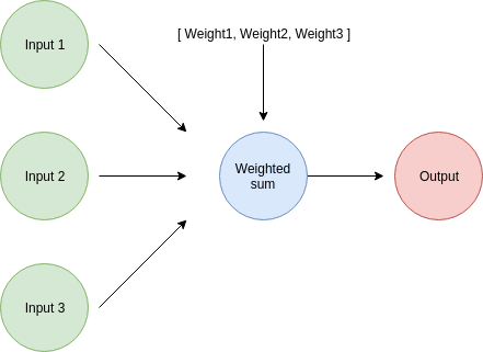
A network with many inputs and only one output has one weight associated with each of the inputs. This means that we will need to calculate the weight correction factor for every single one of them.
    derivative = input * (predicted_value - expected_value)
    weight_adjustment = alpha * derivative

    weight -= weight_adjustment
Or in a more concise way:
    weight_adjustment = input * alpha * (predicted_value - expected_value)
    weight -= weight_adjustment
This is how we calculate the correction factor for every single weight: each weight is responsible for one input, so the calculation for every correction will involve its respective input:
    weight_adjustment_1 =  input_1 * alpha  * (predicted_value - expected_value)
    weight_1 -= weight_adjustment_1

    weight_adjustment_2 =  input_2 * alpha  * (predicted_value - expected_value)
    weight_2 -= weight_adjustment_2

    weight_adjustment_3 =  input_3 * alpha  * (predicted_value - expected_value)
    weight_3 -= weight_adjustment_3
Notice how every adjustment involves a shared part (alpha * (predicted_value - expected_value)) and a specific part that uses the weight and its respective input.
This implementation is obviously not good enough. What happens if we have thousands of inputs? We can easily perform these updates for any number of inputs/weights if we handle them as vectors.
Let’s create methods to calculate the correction factor and to adjust the value of each weight:
def calculate_weight_adjustments(inputs, correction_factor):
    weight_adjustments = []

    for input in inputs:
        weight_adjustment = input * correction_factor
        weight_adjustments.append(weight_adjustment)

    return weight_adjustments


def calculate_updated_weights(weights, weight_adjustments):
    updated_wights = []

    for weight, weight_adjustment in zip(weights, weight_adjustments):
        updated_wight = weight - weight_adjustment
        updated_wights.append(updated_wight)

    return updated_wights
The only ‘weird’ thing in these two methods is correction_factor argument. It’s just a name I gave to the alpha * (predicted_value - expected_value) factor we mentioned before.
With those functions in place, the final implementation is very similar to the base case. Instead of adjusting only one weight at a time, we can adjust the whole weight vector:
    correction_factor = alpha  * (predicted_value - expected_value)
    weight_adjustments = calculate_weight_adjustments(inputs, correction_factor )
    weights = calculate_updated_weights(weights, weight_adjustments)
This is a complete example of gradient descent applied to a multi-input neural network with a single output:
# The 2 functions defined above (calculate_weight_adjustments and calculate_updated_weights) go here

# Our trusty old multi-input neural network implementation
def multi_input_neural_network(inputs, weights):
    assert( len(inputs) == len(weights))

    predicted_value = 0
    for input, weight in zip(inputs, weights):
        predicted_value += input * weight

    return predicted_value

inputs = [0.2, 4, 0.1]
weights = [10, 2, 11]
expected_value = 8
alpha = 0.04

while True:
    # Because of how python handles floating point, we round the values
    predicted_value = round(multi_input_neural_network(inputs, weights), 2)
    print("According to my neural network, the result is {}".format(predicted_value))
    error = (predicted_value - expected_value)**2
    print("The error in the prediction is {} ".format(error))

    correction_factor = alpha  * (predicted_value - expected_value)
    weight_adjustments = calculate_weight_adjustments(inputs, correction_factor )
    print("These are the weight adjustment values: {}".format(weight_adjustments))

    weights = calculate_updated_weights(weights, weight_adjustments)
    print("These are the new weights: {}".format(weights))


    print("\n")
    if(error == 0):
        break
Running this code with an alpha of 0.04 will result in the following learning iteration:
According to my neural network, the result is 11.1
The error in the prediction is 9.609999999999998
These are the weight adjustment values: [0.0248, 0.49599999999999994, 0.0124]
These are the new weights: [9.9752, 1.504, 10.9876]

... More iterations

According to my neural network, the result is 8.01
The error in the prediction is 9.999999999999574e-05
These are the weight adjustment values: [7.999999999999831e-05, 0.001599999999999966, 3.9999999999999156e-05]
These are the new weights: [9.961359999999999, 1.2271999999999998, 10.98068]

According to my neural network, the result is 8.0
The error in the prediction is 0.0
These are the weight adjustment values: [0.0, 0.0, 0.0]
These are the new weights: [9.961359999999999, 1.2271999999999998, 10.98068]
Gradient descent for multiple inputs is easy to understand if you already internalized how it works for the base case. The only difference is that we perform updates on every single weight/input pair.
Gradient descent: Single input - multiple outputs.
Let’s take a look at the opposite case, where we have a neural network with a single input and multiple outputs.
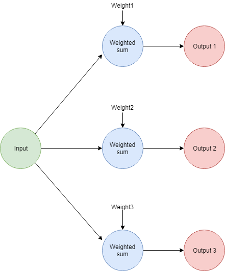
The easiest way of visualizing this scenario is to see every weight/output pair as a single neural network. The main difference is that each one of them will have their own predicted and expected values. Those values will be used to calculate the weight adjustments for the respective sub-network.
This basically means that we are running the 1-input/1-output case 3 times. A naive implementation for the 3-output case looks like this:
    # This happens inside a loop like in the other cases

    # First, we calculate the prediction for every single value
    predicted_value_1 = round(neural_network(input, weight_1), 2)
    predicted_value_2 = round(neural_network(input, weight_2), 2)
    predicted_value_3 = round(neural_network(input, weight_3), 2)

    # Each predicted value will have its own associated prediction error
    error_1 = (predicted_value_1 - expected_value_1)**2
    error_2 = (predicted_value_2 - expected_value_2)**2
    error_3 = (predicted_value_3 - expected_value_3)**2

    # Next, we can use this information to calculate the derivative for each of the 3 cases
    derivative_1 = input * (predicted_value_1 - expected_value_1)
    derivative_2 = input * (predicted_value_2 - expected_value_2)
    derivative_3 = input * (predicted_value_3 - expected_value_3)

    # The information previously calculated is now used to update the value of our weights
    weight_adjustment_1 = alpha * derivative_1
    weight_adjustment_2 = alpha * derivative_2
    weight_adjustment_3 = alpha * derivative_3

    weight_1 -= weight_adjustment_1
    weight_2 -= weight_adjustment_2
    weight_3 -= weight_adjustment_3
The complete implementation (this naive approach) can be found in the article’s source code. Let’s run it to verify it modifies the weights until it correctly predicts the outputs.
According to my neural network, the 1st result is 2.0
According to my neural network, the 2nd result is 4.0
According to my neural network, the 3rd result is 0.6
The error in the 1st prediction is 36.0
The error in the 2nd prediction is 1764.0
The error in the 3rd prediction is 0.25
The value of our derivative for the 1st weight=10 is -1.2000000000000002
The value of our derivative for the 2nd weight=20 is -8.4
The value of our derivative for the 3rd weight=3 is 0.1
The new value of our 1st weight is 38.800000000000004
The new value of our 2nd weight is 221.60000000000002
The new value of our 3rd weight is 0.5999999999999996

... More iterations

According to my neural network, the 1st result is 8.0
According to my neural network, the 2nd result is 46.0
According to my neural network, the 3rd result is 0.1
The error in the 1st prediction is 0.0
The error in the 2nd prediction is 0.0
The error in the 3rd prediction is 0.0
The value of our derivative for the 1st weight=40.00000000000001 is 0.0
The value of our derivative for the 2nd weight=230.00000000000003 is 0.0
The value of our derivative for the 3rd weight=0.5039999999999997 is 0.0
The new value of our 1st weight is 40.00000000000001
The new value of our 2nd weight is 230.00000000000003
The new value of our 3rd weight is 0.5039999999999997
Yes, you are right, this implementation is quite awkward and doesn’t really work beyond 3 outputs. Like before, let’s create some functions that handle all these calculations in vectors:
def calculate_errors(predicted_values, expected_values):
    errors = []
    for pred_value, exp_value in zip(predicted_values, expected_values):
        error = (pred_value - exp_value)**2
        errors.append(error)

    return errors

def calculate_weight_adjustments(alpha, input, predicted_values, expected_values):
    weight_adjustments = []

    for pred_value, exp_value in zip(predicted_values, expected_values):
        weight_adjustment = alpha * input * (pred_value- exp_value)
        weight_adjustments.append(weight_adjustment)

    return weight_adjustments

# calculate_updated_weights is exactly the same as in the multi-input/single-output scenario
With those functions in place, the final implementation is much simpler
# The  functions defined above go here
input = 0.2
alpha = 24

expected_values = [8, 46, 0.1]
weights = [10, 20, 3]

while True:
    # Because of how python handles floating point, we round the values
    predicted_values = neural_network_multi_output(input, weights)

    print("According to my neural network, the 1st result is {}".format(predicted_values[0]))
    print("According to my neural network, the 2nd result is {}".format(predicted_values[1]))
    print("According to my neural network, the 3rd result is {}".format(predicted_values[2]))

    errors = calculate_errors(predicted_values, expected_values)

    print("The error in the 1st prediction is {} ".format(errors[0]))
    print("The error in the 2nd prediction is {} ".format(errors[1]))
    print("The error in the 3rd prediction is {} ".format(errors[2]))

    weight_adjustments = calculate_weight_adjustments(alpha, input, predicted_values, expected_values)

    weights = calculate_updated_weights(weights, weight_adjustments)

    print("The new value of our 1st weight is {}".format(weights[0]))
    print("The new value of our 2nd weight is {}".format(weights[1]))
    print("The new value of our 3rd weight is {}".format(weights[2]))

    print("\n")
    #We stop when all errors are 0
    if(errors[0] + errors[1] + errors[2] == 0):
        break
Running this code produces the same results as the naive implementation we listed above, but the code is much easier to understand and can run with any number of outputs.
A core idea with small changes
As you may have noticed, gradient descent changes very little on the cases we just studied. The main idea is that the topology of the network will change the way we calculate the adjustment factor for the NN’s weights.
If you still don’t feel comfortable with these ideas try to re-implement the code examples on your own. Understanding how we reached the final implementation is a very important pre-requisite for the next article of the series: gradient descent applied to neural networks with any number of inputs and any number of outputs.
Thank you for reading!
What to do next
- Share this article with friends and colleagues. Thank you for helping me reach people who might find this information useful.
- This article is based on the book: Grokking Deep Learning and on Deep Learning (Goodfellow, Bengio, Courville).
- You can find the source code for this series here
- Send me an email with questions, comments or suggestions (it’s in the About Me page)