We already covered the most important deep learning concepts and created different implementations using vanilla Python. Now, we are in a position where we can start building something a bit more elaborate.
We’ll use a more hands-on approach by building a deep learning model for classification using production-grade software.
You will learn how to make a classifier for hand-written digits using Keras, running on top of Tensorflow.
Great, let’s get started!
Before we proceed, what’s Keras?
Keras is a popular library for creating deep learning models.
It’s a high-level API that runs on multiple backends that handle all the processing, like Tensorflow, Theano or Microsoft Cognitive Toolkit.
Since Tensorflow 2 was released, Keras became its official high-level API, so it now comes included by default with the Tensorflow installation.
Setup
Instead of writing instructions that might go outdated I’ll just link to the official resources. You will need to install these:
Good, let’s get started!
Import the libraries and get the data
We can get all the libraries we need with the following lines:
# Import TensorFlow and Keras
import TensorFlow as tf
from tensorflow import keras

# Import support libraries for plotting
import matplotlib.pyplot as plt
Now, let’s get the data. We will use the MNIST set of handwritten digits, one of the most popular datasets for testing ML image classification models. The set includes 60.000 examples for training and 10.000 for testing:
(x_train, y_train), (x_test, y_test) = mnist.load_data()
The load_data method returns two tuples:
- (x_train, y_train) are the 60.000 examples we will use to train the network.
- (x_test, y_test) are the examples we will use to evaluate the performance of the network.
Explore the data
x_train.shape
Output: (60000, 28, 28)

y_train.shape
Output: (60000,)
x_train is a collection of 60.000 28x28 matrices, where each entry in the matrix is a number from 0 to 255. Each 28x28 matrix represents a handwritten number, pixel by pixel. You can visualize them using PyPlot.
# Print the first element in x_train as an image
plt.figure()
plt.imshow(x_train[0])
plt.colorbar()
plt.grid(False)
plt.show()
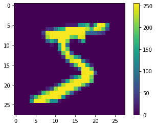
y_train is a collection of 60.000 labels, in this case representing the number its respective x_train element represents. If you recall previous articles, these are the expected values.
Let’s verify the label for the first element is a five:
y_train[0]
Output: 5
Preprocessing the data
Not much is needed for this particular dataset. Neural networks work better if their inputs are between 0 and 1, so let’s perform some normalization on the inputs:
x_train = x_train / 255.0
x_test = x_test / 255.0
These two lines did the trick, we can now start building our network.
Build the network
Now we will build and compile our neural network. In Keras, you only need to define the layers in your network and you are almost done. This is the 8-layer network we will use:
model = keras.Sequential([
    keras.layers.Flatten(input_shape=(28, 28)),
    keras.layers.Dense(512, activation='relu'),
    keras.layers.Dense(216, activation='relu'),
    keras.layers.Dense(128, activation='relu'),
    keras.layers.Dense(64, activation='relu'),
    keras.layers.Dense(32, activation='relu'),
    keras.layers.Dense(16, activation='relu'),
    keras.layers.Dense(10, activation='softmax')
])
Keras has many different types of layers, our network is made of two main types: 1 Flatten layer and 7 Dense layers.
A Flatten layer is used to transform higher-dimension tensors into vectors. In our case, it transforms a 28x28 matrix into a vector with 728 entries (28x28=784).
Dense layers need you to specify the shape of the output (the first parameter) and the activation function. All our layers have relu activation except for the last layer. The output layer uses softmax because that’s the right choice when building a multiclass classifier.
The next step is compiling the model:
model.compile(loss='sparse_categorical_crossentropy',
              optimizer='adam',
              metrics=['accuracy'])
These parameters are:
- loss: Is the optimization score function, the number the network will try to reduce during training.
- optimizer: Is the algorithm used to update the values of the weights in the network.
- metrics: Measurements we perform during training.
You can check the final shape of the network using the .summary() method:
model.summary()

Output:
Model: "sequential"
_________________________________________________________________
Layer (type)                 Output Shape              Param #
=================================================================
flatten (Flatten)            (None, 784)               0
_________________________________________________________________
dense (Dense)                (None, 512)               401920
_________________________________________________________________
dense_1 (Dense)              (None, 216)               110808
_________________________________________________________________
dense_2 (Dense)              (None, 128)               27776
_________________________________________________________________
dense_3 (Dense)              (None, 64)                8256
_________________________________________________________________
dense_4 (Dense)              (None, 32)                2080
_________________________________________________________________
dense_5 (Dense)              (None, 16)                528
_________________________________________________________________
dense_6 (Dense)              (None, 10)                170
=================================================================
Total params: 551,538
Trainable params: 551,538
Non-trainable params: 0
Why did we use a network with this shape? Well, to be honest, because I felt like building one with 9 layers. You can try building a smaller network as an exercise and seeing how the performance changes:
model = keras.Sequential([
    keras.layers.Flatten(input_shape=(28, 28)),
    keras.layers.Dense(216, activation='relu'),
    keras.layers.Dense(10, activation='softmax')
Train the network and evaluate its accuracy
We train the network using the fit() method:
history = model.fit(x_train, y_train, epochs=20, batch_size=15)
The first two arguments are the training examples and their labels, and the third argument is the number of training cycles we will run (in this case 20).batch_size tells you the number of samples that will be propagated through the network before updating the weights. In our network we will update weights every time we process 15 inputs.
Fit returns a history object with information about the trainig process. When you call the fit method you will see the following output:
Train on 60000 samples
Epoch 1/20
60000/60000 [==============================] - 25s 420us/sample - loss: 0.2670 - accuracy: 0.9205
Epoch 2/20
60000/60000 [==============================] - 25s 412us/sample - loss: 0.1127 - accuracy: 0.9670
Epoch 3/20
60000/60000 [==============================] - 26s 440us/sample - loss: 0.0833 - accuracy: 0.9768
Epoch 4/20
60000/60000 [==============================] - 24s 400us/sample - loss: 0.0668 - accuracy: 0.9816
Epoch 5/20
60000/60000 [==============================] - 25s 418us/sample - loss: 0.0579 - accuracy: 0.9838
Epoch 6/20
60000/60000 [==============================] - 36s 606us/sample - loss: 0.0475 - accuracy: 0.9871
Epoch 7/20
60000/60000 [==============================] - 36s 598us/sample - loss: 0.0421 - accuracy: 0.9887
Epoch 8/20
60000/60000 [==============================] - 35s 580us/sample - loss: 0.0356 - accuracy: 0.9905
Epoch 9/20
60000/60000 [==============================] - 32s 534us/sample - loss: 0.0341 - accuracy: 0.9911
Epoch 10/20
60000/60000 [==============================] - 28s 461us/sample - loss: 0.0296 - accuracy: 0.9925
Epoch 11/20
60000/60000 [==============================] - 28s 463us/sample - loss: 0.0289 - accuracy: 0.9927
Epoch 12/20
60000/60000 [==============================] - 28s 459us/sample - loss: 0.0284 - accuracy: 0.9936
Epoch 13/20
60000/60000 [==============================] - 28s 467us/sample - loss: 0.0259 - accuracy: 0.9938
Epoch 14/20
60000/60000 [==============================] - 27s 455us/sample - loss: 0.0259 - accuracy: 0.9938
Epoch 15/20
60000/60000 [==============================] - 29s 486us/sample - loss: 0.0206 - accuracy: 0.9952
Epoch 16/20
60000/60000 [==============================] - 28s 471us/sample - loss: 0.0241 - accuracy: 0.9945
Epoch 17/20
60000/60000 [==============================] - 28s 469us/sample - loss: 0.0211 - accuracy: 0.9952
Epoch 18/20
60000/60000 [==============================] - 28s 461us/sample - loss: 0.0172 - accuracy: 0.9960
Epoch 19/20
60000/60000 [==============================] - 25s 424us/sample - loss: 0.0209 - accuracy: 0.9953
Epoch 20/20
60000/60000 [==============================] - 31s 510us/sample - loss: 0.0170 - accuracy: 0.9959
It tells you epoch by epoch how the values of loss and accuracy change. As expected, every epoch the results become a bit better. If you prefer, you can plot them using PyPlot.
# Plot training & validation accuracy values
plt.plot(history.history['accuracy'])
plt.title('Model accuracy')
plt.ylabel('Accuracy')
plt.xlabel('Epoch')
plt.legend(['Train'], loc='upper left')
plt.show()

# Plot training & validation loss values
plt.plot(history.history['loss'])
plt.title('Model loss')
plt.ylabel('Loss')
plt.xlabel('Epoch')
plt.legend(['Train'], loc='upper left')
plt.show()
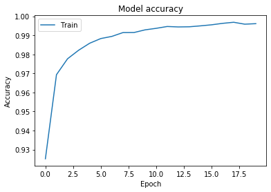
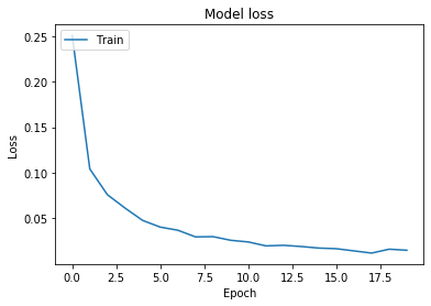
So, we get a final accuracy of 99.61, but you might also remember that evaluating performance on the training set doesn’t make much sense, so let’s try the model on data it hasn’t seen yet.
test_loss, test_acc = model.evaluate(x_test,  y_test, verbose=0)

print('Test accuracy:', test_acc)
print('Test loss:', test_loss)

Output:
Test accuracy: 0.9822
Test loss: 0.14858887433931195
Nice! Accuracy of 98.61% with a loss of 0.01, not bad for our first try on this dataset!
There are many ways of improving these results, but for now, it’s enough to be happy with our hard work.
As we get closer to real-world examples with neural networks, we get closer to the end of this series. In the following article, we will talk about regularization: a series of techniques we can use to fight overfitting in our DL models.
Thank you for reading!
What to do next
- Share this article with friends and colleagues. Thank you for helping me reach people who might find this information useful.
- Try different networks, both bigger and smaller, and see how the size of the network affects performance on both the training and test sets. You can also try training a different amount of epochs.
- Here is the official Keras documentation
- You can find the source code for this series here
- This article is based on the book: Grokking Deep Learning and on Deep Learning (Goodfellow, Bengio, Courville).
- Send me an email with questions, comments or suggestions (it’s in the About Me page)