
In the previous article we learned that neural networks look for the correlation between the inputs and the outputs of a training set. We also learned that based on the pattern, the weights will have an overall tendency to increase or decrease until the network predicts all the values correctly.
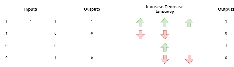
Sometimes there is not a clear direction in this up/down tendency and the network will have trouble learning a pattern. In the following example, each weight is pulled up with the same force it's pulled down.
You can make the test by grabbing our implementation of gradient descent and replacing the data setup section with this one:
# The inputs and expected results are in corresponding order
inputs = nmpy.array([[1,1,1],
                     [1,1,0],
                     [0,1,0],
                     [0,1,1]
                    ])

expected_values = nmpy.array([1,0,1,0])
You can run it and verify it never converges. You could even increase the number of iterations, but it won't help: the network is not able to find a proper correlation between inputs and outputs.
This problem is pretty common, and as you imagined, people already came up with a solution. If the network can't find a clear correlation between inputs and outputs, we can still create an intermediate set that has an actual correlation with the outputs.
This set will be calculated using the inputs. In the world of neural networks, we can do this by creating any number of intermediate layers.
Visualizing multi-layer neural networks
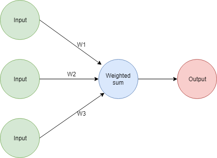
So, let's remember what our network looks like
We can create an additional layer in the network with any number of nodes. The same network with an additional 4-node-layer would look like this:
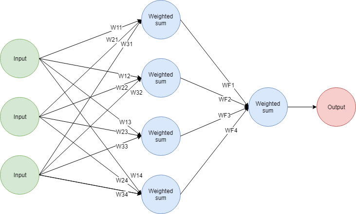
It works like this:
- Every node in the second layer performs a weighted sum of the inputs. It means there are 12 new weights used to produce the inputs of the middle layer.
- The outputs of the 4 nodes in the middle layer work as inputs for the final layer. The final layer performs a weighted sum (so 4 weights used there) and produces an output.
You can see this as two networks stacked together. The outputs of the first part of the network are the inputs for the second part. These additional layers are usually called the hidden layers of the network.
Good, now you understand how the network performs predictions, but how can we adjust the weights? For this, we need to understand a new technique: backpropagation.
Backpropagation: error attribution across layers
Let's remember an important lesson from previous articles: weights are updated based on their contribution to the error in a prediction. Neural networks change the value of their weights in an attempt to reduce their errors.
This is also the reason we multiply by the value of the respective input when calculating the correction factor for a weight. If the input had a value of 0, you can be sure that the weight it was multiplied by did not contribute at all to the overall error in the prediction.
This calculation was pretty straightforward because you could directly associate inputs and weights to the overall error: you had a layer and a dot product, so the calculation was straightforward. But how can we do that when we have multiple layers? How can we correct the values of weights at the beginning of the network?
For that, we need to be able to calculate the error contribution of each weight in the network. The trick is in understanding how the new layer and its weights (WF*) contribute to the final error.
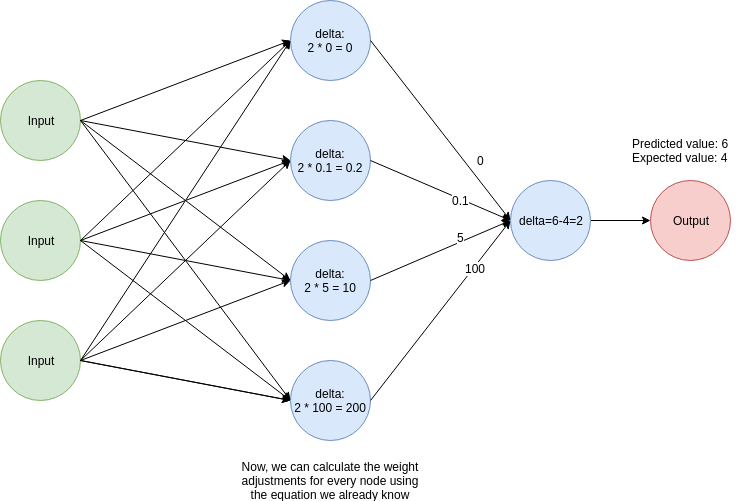
Look for at this network with dummy values:
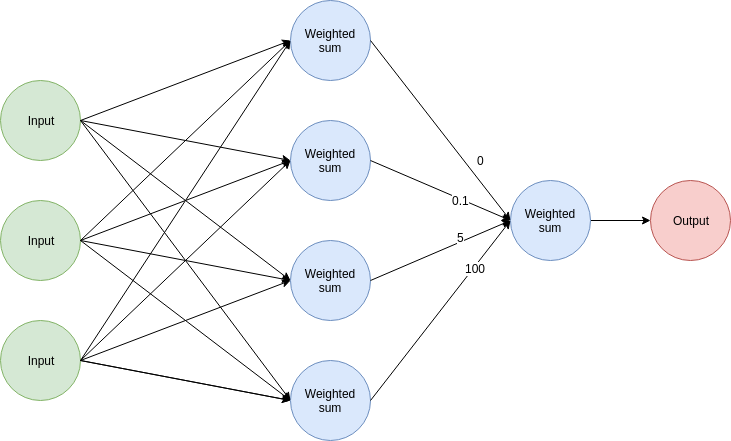
You can make the following assumptions about a prediction:
- The topmost node did not contribute to the overall error because it's associated weight has a value of 0. No matter what value the node had as output, multiplying it by 0 ensures it contributed nothing to the final result.
- The lowermost node had a much bigger contribution than the other nodes due to the high value (100) of its associated weight compared to the others.
So, take a step back and see it from this angle: we can use the values of the weights in that layer as a measurement of how much each node contributed to the overall error.
We can use this idea to calculate the correction factors for the previous layers like this:
- We calculate the value of a delta, which we used in our previous articles to calculate the weight adjustment factors. This is another name for the (predicted_value - expected_value) factor.
- We multiply the value of delta by the values of the weights of the second layer. These values will be used to calculate the weight adjustment factors for the previous layer using the same weight correction equation we've been working with.
Again, this is easier to visualize with an image:
Great! We are almost ready to implement backpropagation in Python. Before writing the complete code, let's have a brief discussion of linearity and activation functions.
Modelling non-linear relations
Here's the thing: it doesn't matter how many layers you add. If all they are doing is a weighted sum you won't gain anything from adding more layers.
The reason is that the dot product is a linear operation. If you have several layers performing a weighted sum, you can always create a one-layer network with the exact same behavior. As an example, look at the following network:
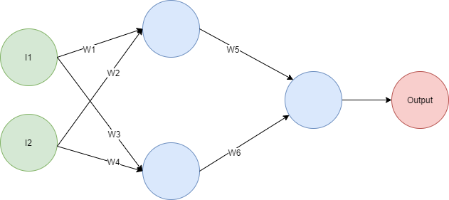
If you do the math you will find out that the output is given by the expression Output = I1(W1W5+W3W6)+I2(W2W5+W4W6), so you can replace it with this network:
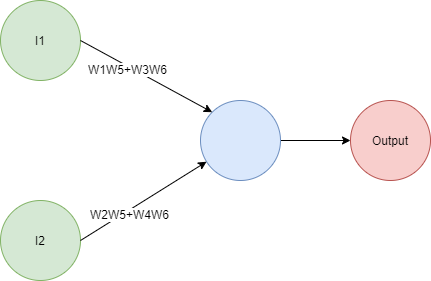
Bigger networks might take a bit more effort to compact by hand due to having a bigger equation, but the same principle applies: no matter how big the network is, you will always be able to replace it with a smaller network.
Remember that originally we wanted to create extra layers to help us build an intermediary representation of our data that has a correlation with the output. What we need is to find a way to bring in some non-linearity into our network to enlarge its hypothesis space. Doing this will help us model much richer behaviors and to create intermediate sets that are not bound to the patterns in the inputs.
We will do this by applying a non-linear activation function to the outputs of each node. There are many different functions we can choose from, but two popular activation functions are relu/rectifier and sigmoid.
In principle, you could use any function as activation function, but not every function will be a good choice. Good activation functions satisfy the following criteria:
- They need to be continuous and their domain must be infinite.
- They need to be monotonic ( not change in direction)
- They need to be non-linear.
- They need to be easy to compute.
For our implementation we will use relu because it's simple and usually yields good results. Given that relu is f(x) we have the following behavior:
- f(x) = 0 if x<0
- f(x) = x if x>=0
In other words, if the output of a node is a number lower than 0 it becomes 0. If it's higher or equal than 0 it forwards the output with no modification.
Now we can use this knowledge to create a complete implementation in Python.
import numpy as nmpy

# These methods run over numpy arrays
def relu(x):
    return (x > 0) * x

def relu_deriv(prev_output):
    return prev_output > 0

# Variable setup: we use numpy's array to create a more concise implementation
alpha = 0.1
hidden_layer_number_of_nodes = 4

weights_1 = nmpy.random.random((3 ,hidden_layer_number_of_nodes))
weights_2 = nmpy.random.random((hidden_layer_number_of_nodes))

inputs = nmpy.array([[1,1,1],
                     [1,1,0],
                     [0,1,0],
                     [0,1,1]
                    ])

expected_values = nmpy.array([1,0,1,0])

run = 0
while True:
    overall_run_error = 0

    for input_set, expected_value in zip(inputs, expected_values):
        # These are the outputs of the intermediate layer (the one with 4 nodes)
        hidden_outputs = relu( nmpy.dot(input_set, weights_1) )
        # This is the final output, this concludes the prediction process
        predicted_value = round(nmpy.dot(hidden_outputs, weights_2), 1)

        # Now, we calculate the deltas and update the weights using
        # the logic we previously described
        layer2_delta = (predicted_value - expected_value)
        # relu_deriv makes sure we only update nodes with output > 0
        layer1_delta = (weights_2 * layer2_delta) * relu_deriv(hidden_outputs)

        weights_2 -= alpha * hidden_outputs.dot(layer2_delta)
        weights_1 -= alpha * nmpy.outer(input_set, layer1_delta)

        # We calculate an accumulated error for every run
        overall_run_error += nmpy.sum((predicted_value-expected_value) ** 2)

    run += 1
    ## Let's print some debug data
    print("The weights in the final layer are: \n{}".format(weights_2) )
    print("The weights in the first layer are: \n{}".format(weights_1) )
    print("The overall error for the run {} is {}\n\n".format(run, overall_run_error))

    if overall_run_error == 0:
        break
Run the code to verify it converges to a solution with 0 error:
The weights in the final layer are:
[ 0.13677727  0.29952828 -0.09968558  0.56497112]
The weights in the first layer are:
[[ 0.68186112 -0.07723001  0.61481898  0.01363698]
 [ 0.28297269 -0.07377539  0.00576834  0.54298254]
 [ 0.57557199  0.41983547  0.57342688  0.13776574]]
The overall error for the run 1 is 4.95


The weights in the final layer are:
[ 0.10819863  0.28437992 -0.12201187  0.54867314]
The weights in the first layer are:
[[ 0.67741254 -0.06524888  0.6134278   0.0065985 ]
 [ 0.27715933 -0.08351396  0.00435572  0.53331793]
 [ 0.56920599  0.4100969   0.5751969   0.11835256]]
The overall error for the run 2 is 1.39

...

The weights in the final layer are:
[-0.26000191  1.74695864 -0.55762033  1.03700425]
The weights in the first layer are:
[[ 0.4874603   1.06748941  0.5756712  -0.46733342]
 [ 0.07043213 -1.10048561 -0.00235896  0.9503538 ]
 [ 0.45488944  1.09249163  0.63419715 -0.44475593]]
The overall error for the run 147 is 0.019999999999999997


The weights in the final layer are:
[-0.26000191  1.74695864 -0.55762033  1.03700425]
The weights in the first layer are:
[[ 0.4874603   1.06748941  0.5756712  -0.46733342]
 [ 0.07043213 -1.10048561 -0.00235896  0.9503538 ]
 [ 0.45488944  1.09249163  0.63419715 -0.44475593]]
The overall error for the run 148 is 0.0
Deep learning, deep networks
Now we know all the fundamental pieces needed to understand deep learning. The main difference between traditional NNs and modern deep learning architectures is the sheer number of layers.
Until recently training networks with huge numbers of inputs and layers was not possible, but thanks to powerful computers and the ingenuity of computer scientists we can now solve novel problems using this powerful idea.
Deep down, deep-learning architectures build intermediate representations of the inputs that model the presence or absence of particular features. Think of a network tasked with identifying the faces of dogs, such a network will probably have intermediate layers detecting the presence of dog noses, ears, and eyes, among many other features. A final layer takes into consideration all the previous results to emit a verdict.
Thank you for reading!
What to do next
- Share this article with friends and colleagues. Thank you for helping me reach people who might find this information useful.
- You can find the source code for this series in this repo.
- This article is based on Grokking Deep Learning and on Deep Learning (Goodfellow, Bengio, Courville). These and other very helpful books can be found in the recommended reading list.
- Send me an email with questions, comments or suggestions (it's in the About Me page)