
In the previous article we learned how to use Keras to build more powerful neural networks. Professional-grade libraries like Keras, Tensorflow, and Pytorch let you build neural networks that can learn intricate patterns and solve novel problems.
Deep-learning networks lets learn subtle patterns thanks to their inherently large hypothesis space, but this brings a new problem: overfitting. Neural networks are prone to overfit, so it's important to know the basics of regularization.
What's regularization? It's a set of techniques used to ease the problem of overfitting. In this article, we will learn how to detect and fix overfitting in our neural networks.
If you are not familiar with the terms overfitting and validation/test sets, take a look at these articles before proceeding:
Good, let's get started!
Detecting overfitting
We'll use a very similar setup to one we used in the previous article: A Keras NN that tries to classify the MNIST set of handwritten digits.
# Import tensorflow and Keras
import tensorflow as tf
from tensorflow import keras

# Import support libraries for matrix operations and plotting
import numpy as np
import matplotlib.pyplot as plt

# Get the MNIST dataset
from keras.datasets import mnist
(x_train, y_train), (x_test, y_test) = mnist.load_data()

# Scale the inputs
x_train = x_train / 255.0
x_test = x_test / 255.0
This part is the same as in the last article.
Now we will extract our validation set from the training examples. To make the effects of overfitting more visible, we will train the network using a limited set of data: only 450 examples. For validation, we will use the last 20.000 examples of the original training set.
x_validation = x_train[40000:]
y_validation = y_train[40000:]

x_train = x_train[:450]
y_train = y_train[:450]
This is our network:
model = keras.Sequential([
    keras.layers.Flatten(input_shape=(28, 28)),
    keras.layers.Dense(128, activation='relu'),
    keras.layers.Dense(64, activation='relu'),
    keras.layers.Dense(32, activation='relu'),
    keras.layers.Dense(16, activation='relu'),
    keras.layers.Dense(10)
])

model.compile(optimizer='rmsprop',
              loss=tf.keras.losses.SparseCategoricalCrossentropy(from_logits=True),
              metrics=['accuracy'])

model.summary()

Output:
Model: "sequential"
_________________________________________________________________
Layer (type)                 Output Shape              Param #
=================================================================
flatten (Flatten)            (None, 784)               0
_________________________________________________________________
dense (Dense)                (None, 128)               100480
_________________________________________________________________
dense_1 (Dense)              (None, 64)                8256
_________________________________________________________________
dense_2 (Dense)              (None, 32)                2080
_________________________________________________________________
dense_3 (Dense)              (None, 16)                528
_________________________________________________________________
dense_4 (Dense)              (None, 10)                170
=================================================================
Total params: 111,514
Trainable params: 111,514
Non-trainable params: 0
Now it's time to train it. This is where we use our validation data, we feed it as a tuple in the validation_data argument of the fit method
history = model.fit(x_train, y_train, epochs=30, validation_data=(x_validation, y_validation), batch_size=15)
Now we can see if our network overfits. For that, we will check how the value of the loss changes after every epoch.
# Plot training & validation accuracy values
plt.plot(history.history['loss'])
plt.plot(history.history['val_loss'])
plt.title('Model loss')
plt.ylabel('Loss')
plt.xlabel('Epoch')
plt.legend(['Train', 'Validation'], loc='upper left')
plt.show()
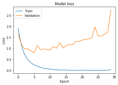
After every learning cycle, our network evaluates its performance on the validation and training sets. Ideally, both the training and validation loss would go down after every epoch, but if the networks overfits, the validation loss will start to go up.
This happens when the network starts to learn quirks in the training set that don't really represent general patterns that apply to unseen data. This causes the network's performance to drop the more we train it.
If you pay attention to our plot you can notice how the network starts to overfit around the 5th epoch. Before we study solutions let's evaluate the network on our test set.
test_loss, test_acc = model.evaluate(x_test,  y_test, verbose=2)

print('Test accuracy:', test_acc)
print('Test loss:', test_loss)

Output:
10000/10000 - 1s - loss: 2.8394 - accuracy: 0.7328
Test accuracy: 0.7328
Test loss: 2.8394393890172243
Our baseline is accuracy of 0.73 and a loss of 2.83, let's see if we can do better.
First solution: Early stopping
The simplest way to prevent overfitting is to stop the training process earlier. It works because networks usually learn the broadest features in the dataset before it starts to learn the noise.
In practice doing this is very easy. In our base example we ran 30 epochs, let's bring that down to 9 epochs and see if it improves things.
history = model.fit(x_train, y_train, epochs=9, validation_data=(x_validation, y_validation), batch_size=15)
Now, let's plot the loss values:
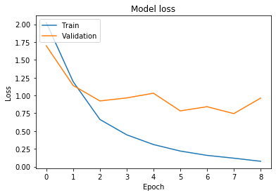
You can notice that in the last epochs the loss in the validation set starts to climb, but it never grows as much as in the base case. We can also check the performance of the network on the training set to see if there was an improvement.
test_loss, test_acc = model.evaluate(x_test,  y_test, verbose=2)

print('Test accuracy:', test_acc)
print('Test loss:', test_loss)

Output:
10000/10000 - 1s - loss: 0.9608 - accuracy: 0.7559
Test accuracy: 0.7559
Test loss: 0.9607989938259125
We had a modest improvement in accuracy, from 0.73 to 0.75, and our loss went from 2.83 to 0.96, not bad if you consider all we did was reducing the number of epochs!
Let's try another simple solution: reducing the complexity of our network.
Second solution: Reduce the complexity of the network
If our network is learning too much noise from the training set, trying a smaller network might help. A smaller network has a more constrained hypothesis space, so it's more likely that it will focus on learning general patterns and neglect quirks in the data.
Instead of using our base network, let's try this one:
# Let's now build the model

model = keras.Sequential([
    keras.layers.Flatten(input_shape=(28, 28)),
    keras.layers.Dense(32, activation='relu'),
    keras.layers.Dense(10)
])

model.compile(optimizer='rmsprop',
              loss=tf.keras.losses.SparseCategoricalCrossentropy(from_logits=True),
              metrics=['accuracy'])

model.summary()

Output:
Model: "sequential_2"
_________________________________________________________________
Layer (type)                 Output Shape              Param #
=================================================================
flatten_2 (Flatten)          (None, 784)               0
_________________________________________________________________
dense_10 (Dense)             (None, 32)                25120
_________________________________________________________________
dense_11 (Dense)             (None, 10)                330
=================================================================
Total params: 25,450
Trainable params: 25,450
Non-trainable params: 0
__________________________
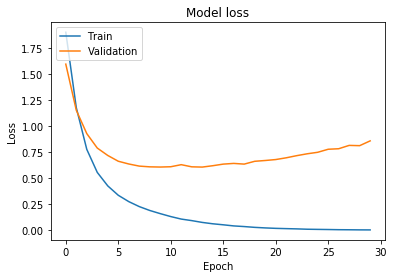
Our trainable parameters now are only 25.450, down from the original 111.514. We will train it for 30 epochs like in the base case.
history = model.fit(x_train, y_train, epochs=30, validation_data=(x_validation, y_validation), batch_size=15)
And, like in the previous case, plot the loss and evaluate the performance on the training set.
test_loss, test_acc = model.evaluate(x_test,  y_test, verbose=2)

print('Test accuracy:', test_acc)
print('Test loss:', test_loss)

Output:
10000/10000 - 0s - loss: 0.8094 - accuracy: 0.8216
Test accuracy: 0.8216
Test loss: 0.8094104566439986
You can notice the loss is now climbing in a much softer way, our accuracy improved and our loss diminished. Again, pretty good results for doing less work than in our base case.
Third solution: Use dropout
The last technique we will use is maybe the most elaborate one: the use of dropout layers in our network.
Dropout layers 'turn off' a percentage of the nodes during training. This means that you will only train randomized subsections of the network on every weight update.
Why does this work? The principle is very similar to what happens with ensemble models: you train different models and use an aggregate result from them to produce predictions. The errors of all the models cancel each other out and in the end, you get better results.
By independently training subsections of the network we end up with a final model that is less prone to overfitting and generalizes better. How do you implement this in Keras? There is a special layer called Dropout that receives as parameter the percentage of weights it must turn off.
Let's build a network that uses 3 Dropout layers on top of our base model:
model = keras.Sequential([
    keras.layers.Flatten(input_shape=(28, 28)),
    keras.layers.Dropout(0.2),
    keras.layers.Dense(128, activation='relu'),
    keras.layers.Dense(64, activation='relu'),
    keras.layers.Dropout(0.2),
    keras.layers.Dense(32, activation='relu'),
    keras.layers.Dense(16, activation='relu'),
    keras.layers.Dropout(0.5),
    keras.layers.Dense(10)
])

model.compile(optimizer='rmsprop',
              loss=tf.keras.losses.SparseCategoricalCrossentropy(from_logits=True),
              metrics=['accuracy'])

Output:
model.summary()
Model: "sequential_3"
_________________________________________________________________
Layer (type)                 Output Shape              Param #
=================================================================
flatten_3 (Flatten)          (None, 784)               0
_________________________________________________________________
dropout (Dropout)            (None, 784)               0
_________________________________________________________________
dense_12 (Dense)             (None, 128)               100480
_________________________________________________________________
dense_13 (Dense)             (None, 64)                8256
_________________________________________________________________
dropout_1 (Dropout)          (None, 64)                0
_________________________________________________________________
dense_14 (Dense)             (None, 32)                2080
_________________________________________________________________
dense_15 (Dense)             (None, 16)                528
_________________________________________________________________
dropout_2 (Dropout)          (None, 16)                0
_________________________________________________________________
dense_16 (Dense)             (None, 10)                170
=================================================================
Total params: 111,514
Trainable params: 111,514
Non-trainable params: 0
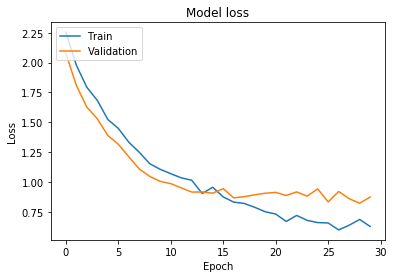
And train it for 30 epochs
history = model.fit(x_train, y_train, epochs=30, validation_data=(x_validation, y_validation), batch_size=15)
These are the results:
test_loss, test_acc = model.evaluate(x_test,  y_test, verbose=2)

print('Test accuracy:', test_acc)
print('Test loss:', test_loss)

Output:
10000/10000 - 1s - loss: 0.8912 - accuracy: 0.8258
Test accuracy: 0.8258
Test loss: 0.891159076166153
Nice! We obtained better results than in our base case, and the loss curve makes us wonder if the network can still be trained for more epochs before it overfits.
Using Dropout is a very popular method with convolutional neural networks and image processing with NNs. If you are interested in these topics being familiar with dropout will come in handy.
Is that all?
Well, why don't you experiment a bit? Grab this article's code and try the following:
- Train the network for less than 9 epochs. What are the results if you train it for 5 epochs? What about 3?
- Try a smaller network, or try different numbers of layers and sizes and compare the results.
- Use dropout layers with different percentages, try 0.1, or 0.3. Put them in different places and see how it affects the results.
- Try different combinations of all these approaches, have fun!
Regularization is a very important topic, central to production-ready solutions that use neural networks. Like most things in this field it's one part science and one part art, so keep running experiments until you get the hang of it.
The next article will be the last in this series. We will discuss some final considerations and offer some pointers to continue learning about this fascinating topic.
Thank you for reading!
What to do next
- Share this article with friends and colleagues. Thank you for helping me reach people who might find this information useful.
- Here is the official Keras documentation
- You can find the source code for this series in this repo.
- This article is based on Grokking Deep Learning and on Deep Learning (Goodfellow, Bengio, Courville). These and other very helpful books can be found in the recommended reading list.
- Send me an email with questions, comments or suggestions (it's in the About Me page)