In previous articles, we learned how neural networks adjust their weights to improve the accuracy of their predictions using techniques like gradient descent.
In this article, we will take a look at the learning process using a more abstract perspective. We will discuss the correlation between inputs and outputs in a training set, and how neural networks find patterns in data.
Hi, my name is Guinea Piggie
We will use a hypothetical experiment as background to learn about correlation. Suppose you form part of an experiment whose goal is... well I can't think about any reason other than torturing you. The experiment is quite simple:
In front of you, there are three buttons (red, green, and blue) and a lever. You are asked to press down any button configuration and then pull the lever. For some configurations, you get an electric shock, and for others you get candy. You are asked to find a pattern by trial and error.
After playing with the system for a while (and suffering several electric shocks), you write down the following pattern:
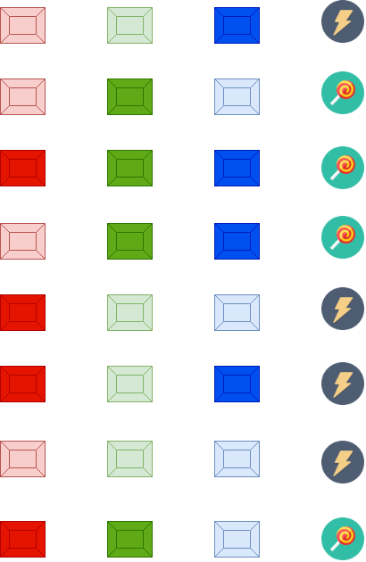
Each row in the image represents a combination of buttons and their respective result. In the first row, for example, only the blue-button was pressed and you received an electric shock. In the third row, you pressed every button and received candy instead.
We want to train a neural network to play this game. When given information about which buttons were pressed it will predict the result, be it candy or electric shock.
Feeding patterns
Our neural network will perform a very simple action: it will map a pattern of inputs into outputs. Deep down, this is what neural networks do: map a set of inputs to a set of outputs.
We have a complete data set for training our network, but networks don't understand button colors or the difference between being electrocuted or having candy. We need to transform our training data into a form that our network can understand.
The most common way of doing this is by creating a matrix that represents the same pattern, like this one:
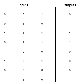
In our matrix representation for the inputs, the value 1 means the button was pressed and 0 means it wasn't pressed. The first column represents the red button, the middle column represents the green one and the right column the blue one.
In our outputs column, we represent the electric shock with a 0 and the candy with a 1.
There are other ways of representing this pattern, you could, for example, write the following matrix:
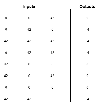
There is an infinite number of matrices that codify this same pattern, which leads us to a very important realization: neural networks don't understand the data they are fed, they just find a mapping between the pattern in the inputs and the pattern in the outputs.
It's up to the human being using the network to find out the meaning of the results. As long as you find a consistent way of representing inputs and outputs, the network will do its best to find a mapping.
Learning correlation by error attribution
The next step is understanding how neural networks learn the correlation.
The title kind of says it: a neural network calculates an error and then updates weights to bring the error down to 0. We studied in previous articles how to use gradient descent to update the value of weights in the right direction (raise or lower their value).
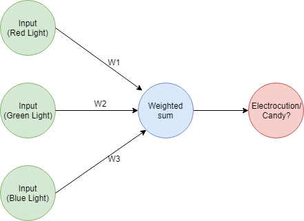
Remember that a neural network performs a weighted sum using the input and weight vectors. After calculating the error it proceeds to update the weights in the hopes of bringing down the error value. In this update step, 3 things can happen:
- The weights that multiplied inputs with a positive correlation with the output increase in value. This is a form of giving more importance to those inputs and to enable them to pull the prediction in the direction of the expected value.
- The weights that multiplied inputs with a negative correlation with the output decrease in value. This is a form of protecting the prediction from being influenced by the inputs that pull it away from the expected value.
- If the weight multiplied an input with a value of 0, nothing happens. Such inputs could not have affected the prediction, so no update in the weights is needed.
Aside from the direction of the update, there is another important mechanism to attribute error to a particular input. Remember the weight updating factor is calculated as alpha * input * (predicted_value - expected_value), notice that the whole expression is multiplied by input.
If the value of the input is high and the error is also high, we can assume that the individual contribution of that input to the error was big, and update accordingly. On the other hand, if the input had a value of 0, we know that particular input contributed nothing to the error.
We can perform an informal analysis with the inputs and outputs and understand the direction in which weights are updated. Let's see our first example, corresponding to the 4th row in the matrix. In this case, we have:
- Red light was off (0)
- Green light was on (1)
- Blue light was on (1)
- We got candy (1)
We know that the red light contributed nothing to the error, so it's associated weight doesn't need to change. Green and blue light, on the other hand, both contributed to the result and have a positive correlation with it (1). Because of this, we know that the value of their associated weights should be pushed upwards.
Let's now check row number six, where we got:
- Red light was on (1)
- Green light was off (0)
- Blue light was on (1)
- We got an electric shock (0)
We know that the green light contributed nothing because it was a 0, so no change to its weight. But now, both red light and blue light contributed to the result of 0 with a negative correlation. In this scenario, the weights associated with red and blue should be pushed downwards.
You can create an additional matrix showing the tendency to increase or decrease the weights:
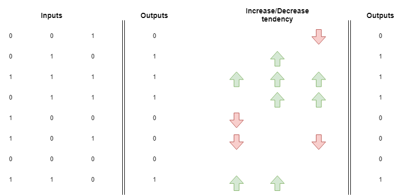
If you average these you will notice that the weight for the green input has a tendency to go up. This means that after training a neural network with all these examples the green light will have a weight with a higher value than the red and blue lights.
What this means is that there is a high positive correlation between pressing the green light and getting candy
This oversimplified representation lets you forget about the complexities of gradient descent and just concentrate on a simple fact: learning rewards inputs that are correlated to specific outputs by assigning them larger weights.
This example is a bit different from the previous regarding the size of the training set. In previous articles, we had only one example we optimized for, whereas now we have 8 of them. Let's learn how to use gradient descent to train a neural network with more than one item in the training set.
Stochastic gradient descent
Stochastic gradient descent is just a fancy term that means run gradient descent for every example in the training set and update weights accordingly.
It works like this:
- Grab the first example in the training set.
- Make a prediction, calculate the error and update the weights
- Perform (1) and (2) again with the second item in the training set, then the third, and so on. Run this cycle until the network predicts the outputs well enough for every input.
In the previous articles, we implemented all our networks from scratch using only Python's standard features.
We will now implement our network using a popular library called NumPy. It will handle matrix and vector operations for us resulting in a more concise implementation.
First, let's set up the variables. All vectors and matrices will be NumPy arrays:
import numpy as nmpy

# Variable setup: we use NumPy's array to create a more concise implementation
alpha = 0.1
weights = nmpy.array([0.5, 0.5, 0.5])

# The inputs and expected results are in corresponding order
inputs = nmpy.array([[0,0,1],
 [0,1,0],
 [1,1,1],
 [0,1,1],
 [1,0,0],
 [1,0,1],
 [0,0,0],
 [1,1,0]
 ])

expected_values = nmpy.array([0,1,1,1,0,0,0,1])
Now, let's implement the weight-adjustment loop.
Because we are performing the stochastic version of gradient descent, we will perform runs that train the network with every element in the training set. In this case, we will run the cycle 15 times.
The implementation will be much more concise than in previous examples because NumPy will handle all vector/matrix operations for us.
# Let's run the optimization for every input 15 times
for run in range(15):
 # This is the total error of a single run
 error_for_run = 0
 # Now we apply gradient descent to every pair of inputs/expected values
 for input_set, expected_value in zip(inputs, expected_values):

 # We can calculate our predicted value with a simple dot product operation, neat!
 predicted_value = round( input_set.dot(weights), 1)
 print("Our network predicted {} for the inputs {}".format(predicted_value, input_set))

 # Error calculation is the same as before, but with NumPy magic!
 error = (predicted_value - expected_value) ** 2
 error_for_run += error

 # With the magic of NumPy, updating weights is this easy!
 weights -= alpha * (input_set * (predicted_value - expected_value) )

 print("The accumulated error for this run is {} \n\n\n".format(error_for_run))
Notice the following:
- We keep the overall error for every single run, whose value is the sum of the errors in the prediction of every element in the set.
- The predicted value is just a dot product between the inputs and the weights. We round to 1 decimal place for convenience.
- The error calculation and weight updates use NumPy's overloaded operators for addition, subtraction, and multiplication. Remember how much code it required in previous articles? That's the power of using libraries specially designed for these tasks.
You can verify this code performs the correct weight adjustment by running it and inspecting the results:
Our network predicted 0.5 for the inputs [0 0 1]
Our network predicted 0.5 for the inputs [0 1 0]
Our network predicted 1.5 for the inputs [1 1 1]
Our network predicted 0.9 for the inputs [0 1 1]
Our network predicted 0.4 for the inputs [1 0 0]
Our network predicted 0.8 for the inputs [1 0 1]
Our network predicted 0.0 for the inputs [0 0 0]
Our network predicted 0.8 for the inputs [1 1 0]
The accumulated error for this run is 1.6


Our network predicted 0.3 for the inputs [0 0 1]
Our network predicted 0.5 for the inputs [0 1 0]
Our network predicted 1.2 for the inputs [1 1 1]
Our network predicted 0.8 for the inputs [0 1 1]
Our network predicted 0.3 for the inputs [1 0 0]
Our network predicted 0.6 for the inputs [1 0 1]
Our network predicted 0.0 for the inputs [0 0 0]
Our network predicted 0.8 for the inputs [1 1 0]
The accumulated error for this run is 0.9099999999999999

... more iterations ...

Our network predicted 0.0 for the inputs [0 0 1]
Our network predicted 0.9 for the inputs [0 1 0]
Our network predicted 1.0 for the inputs [1 1 1]
Our network predicted 1.0 for the inputs [0 1 1]
Our network predicted 0.0 for the inputs [1 0 0]
Our network predicted 0.0 for the inputs [1 0 1]
Our network predicted 0.0 for the inputs [0 0 0]
Our network predicted 1.0 for the inputs [1 1 0]
The accumulated error for this run is 0.009999999999999995


Our network predicted 0.0 for the inputs [0 0 1]
Our network predicted 1.0 for the inputs [0 1 0]
Our network predicted 1.0 for the inputs [1 1 1]
Our network predicted 1.0 for the inputs [0 1 1]
Our network predicted 0.0 for the inputs [1 0 0]
Our network predicted 0.0 for the inputs [1 0 1]
Our network predicted 0.0 for the inputs [0 0 0]
Our network predicted 1.0 for the inputs [1 1 0]
The accumulated error for this run is 0.0
Cool, now we know how to implement stochastic gradient descent!
Sometimes one layer is not enough
We were lucky with our training set because there was a clear correlation between inputs and outputs.
The green button had a very strong correlation with the candy result. The red and blue button didn't have a clear tendency, so the network had to wait until the green light's weight converged to a value to correct both these other button's weights. When the green light was generating the right results, both the red and blue light absorbed all the error in the prediction, and the correction was possible.
Sometimes the training set doesn't have such clear patterns. What happens if for example all of them have the same tendency to raise and decrease? In this scenario, it's possible to build intermediate layers in the network that actually do have a correlation with the output.
This is the foundation of deep learning: multi-layer neural networks. Building networks with many layers will let you solve problems that smaller networks are not able to. Of course, this comes with challenges: how do you attribute error to layers in the first stages of the prediction?
This has a solution: backpropagation. In the next article, we will learn how neural networks with many layers use this technique to correctly update the weights across the whole network.
What to do next
- Share this article with friends and colleagues. Thank you for helping me reach people who might find this information useful.
- You can find the source code for this series in this repo.
- This article is based on Grokking Deep Learning and on Deep Learning (Goodfellow, Bengio, Courville). These and other very helpful books can be found in the recommended reading list.
- Send me an email with questions, comments or suggestions (it's in the About Me page)